Lecture 2: Optimum Design Problem Formulation

In our last lecture, we established the fundamental concepts of design optimization and differentiated it from traditional design and analysis. Today, we delve into a crucial aspect of optimum design: Problem Formulation. This is the step where we translate a descriptive engineering design challenge into a precise mathematical optimization problem. A well-formulated problem is the foundation for finding the best possible solution, so understanding this process is absolutely vital for any aspiring design engineer.

By the end of this lecture, you will be able to translate a descriptive statement of a design problem into a mathematical statement for optimization, identifying and defining its key components: design variables, optimization criterion, and constraints.

The Problem Formulation Process

Formulating an optimum design problem involves a systematic, step-by-step approach. It’s essentially about asking the right questions and expressing the answers in a rigorous mathematical language.

Step 1: Project/Problem Description

The formulation process begins with a clear, descriptive statement of the project or problem. This statement, often provided by a project owner or sponsor, outlines the overall objectives and specific requirements that the system must meet. It’s about understanding what needs to be designed and why.

Example: “Design a new, lightweight casing for a portable electronic device. The casing must be robust enough to withstand a drop from 1 meter without damage, have a smooth external finish, and be manufacturable using injection molding. The primary goal is to minimize the total weight of the casing.”

Step 2: Data and Information Collection

Once the problem is clearly described, the next step is to gather all necessary data and relevant analysis expressions. This includes material properties, external loads, environmental conditions, geometric limitations, manufacturing processes, and any equations or formulas needed to analyze the system’s performance (e.g., stress calculations, deflection formulas, volume, mass equations). Without accurate data, even a perfectly formulated problem cannot lead to a meaningful solution.

Example (for the electronic device casing): * Material properties: Density (\(\rho\)), Young’s modulus (E), Yield strength (\(\sigma_y\)) for potential plastics. * Load conditions: Impact force from a 1-meter drop. * Manufacturing limits: Minimum wall thickness for injection molding. * Geometric space: Maximum external dimensions for the casing. * Equations: Formulas for calculating stress, deflection, and mass based on geometry.

Step 3: Definition of Design Variables

Design variables are the fundamental parameters that the designer can change to influence the system’s performance. They are the “knobs” that you, as the engineer, can adjust. These variables are typically represented as an n-dimensional vector, x = (x1, x2, …, xn).

Key considerations for defining design variables:

Independence: Ideally, design variables should be as independent of each other as possible. If variables are highly dependent, it can complicate the optimization process.
Completeness: The chosen design variables should fully define the system such that its performance can be evaluated.
Influence: They should be parameters that have a significant impact on the objective function and constraints.

Example (for the electronic device casing): If the casing is a simple rectangular box, design variables could be: * x1 = length of the casing * x2 = width of the casing * x3 = height of the casing * x4 = wall thickness of the casing

Step 4: Optimization Criterion (Objective Function)

The optimization criterion, or objective function, is a single scalar measure of the design’s performance that you want to either minimize or maximize. It quantifies the “goodness” of a design. It must be expressed as a function of the design variables, f(x).

Common objectives in mechanical engineering:

Minimize: Mass, cost, energy consumption, stress, deflection, vibration, manufacturing time.
Maximize: Efficiency, strength, stiffness, lifespan, profit, reliability, ride quality.

Sometimes, a problem may seem to have multiple objectives (e.g., minimize weight and minimize cost). Such problems are called multiobjective design optimization problems, and they require specialized techniques (which we will briefly touch upon later in the course). For now, we will focus on problems with a single, clearly defined objective.

Example (for the electronic device casing): To minimize the total mass of the casing. Assuming a simple hollow rectangular box, the mass (M) could be approximated as: M = \(\rho\) * (Volume of solid material) If the outer dimensions are \(L_o\), \(W_o\), \(H_o\) and wall thickness is \(t\): Volume = \((L_o W_o H_o) - ((L_o - 2t)(W_o - 2t)(H_o - 2t))\) So, \(f(x_1, x_2, x_3, x_4)\) = \(\rho \times (x_1 x_2 x_3 - (x_1 - 2x_4)(x_2 - 2x_4)(x_3 - 2x_4))\)

Step 5: Formulation of Constraints

Constraints are limitations or restrictions on the design variables or the system’s performance. They arise naturally in almost all engineering problems and ensure that the final design is practical, safe, and meets all functional requirements. Constraints are expressed mathematically as equalities or inequalities involving the design variables.

Types of constraints:

Performance Constraints: Related to the behavior of the system (e.g., stress must not exceed allowable stress, deflection must be less than a certain limit).
- Inequality: \(g_j(x) \le 0\)
- Equality: \(h_k(x) = 0\)
Geometric Constraints: Limitations on dimensions (e.g., width must be less than length, minimum clearance).
Resource Constraints: Limitations on available materials, budget, manufacturing capacity.
Side Constraints (Bounds on Variables): Simple upper and lower limits on each design variable.
- \(x_{iL} \le x_i \le x_{iU}\)

It is a common practice to convert all inequality constraints into the “less than or equal to zero” form (\(g_j(x) \le 0\)) for standardization. If a constraint is originally \(G(x) \ge C\), it can be rewritten as \(C - G(x) \le 0\).

Example (for the electronic device casing):

Material Strength Constraint: Maximum stress (\(\sigma_{max}\)) must not exceed the material’s yield strength (\(\sigma_y\)). This will depend on the impact load and geometry. \(g_1(x_1, x_2, x_3, x_4) = \sigma_{max}(x_1, x_2, x_3, x_4) - \sigma_y \le 0\)
Deflection Constraint: Maximum deflection (\(\delta_{max}\)) must not exceed a specified limit (\(\delta_{allow}\)). \(g_2(x_1, x_2, x_3, x_4) = \delta_{max}(x_1, x_2, x_3, x_4) - \delta_{allow} \le 0\)
Width-to-thickness ratio: To avoid local buckling or ensure manufacturability. \(g_3(x_2, x_4) = \frac{x_2}{x_4} - \text{ratio}_{max} \le 0\)
Side Constraints (Bounds on Variables): \(x_{1L} \le x_1 \le x_{1U}\) (e.g., 50 mm \(\le x_1 \le\) 200 mm) \(x_{2L} \le x_2 \le x_{2U}\) (e.g., 30 mm \(\le x_2 \le\) 100 mm) \(x_{3L} \le x_3 \le x_{3U}\) (e.g., 10 mm \(\le x_3 \le\) 50 mm) \(x_{4L} \le x_4 \le x_{4U}\) (e.g., 1 mm \(\le x_4 \le\) 5 mm)

General Mathematical Model for Optimum Design

Combining all these steps, a general mathematical model for an optimum design problem can be stated as:

Find the design variable vector \(\mathbf{x} = (x_1, x_2, ..., x_n)\)

To minimize (or maximize) the objective function \(f(\mathbf{x})\)

Subject to: * Equality constraints: \(h_k(\mathbf{x}) = 0\), for \(k = 1, ..., p\) * Inequality constraints: \(g_j(\mathbf{x}) \le 0\), for \(j = 1, ..., m\) * Side constraints (bounds): \(x_{iL} \le x_i \le x_{iU}\), for \(i = 1, ..., n\)

The set of all design points x that satisfy all these constraints is known as the feasible set or feasible design space. Our goal is to find the point within this feasible set that gives the best (minimum or maximum) value for the objective function.

Solved Examples

Let’s apply this formulation process to a few engineering design problems.

Example 1: Minimum-Weight Tubular Column Design

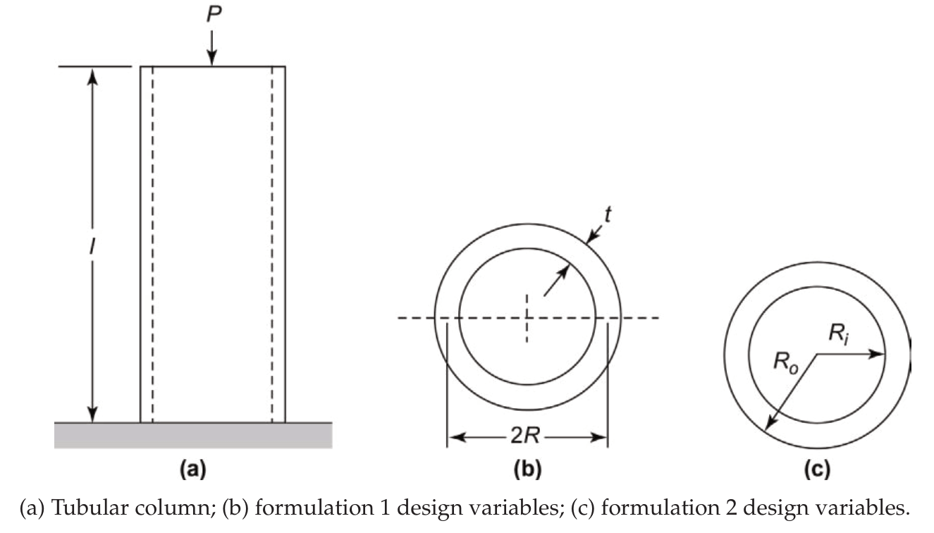
Step 1: Project/Problem Description Design a minimum-mass tubular column of length \(L\) supporting an axial load \(P\) without buckling or overstressing. The column is fixed at the base and free at the top (a cantilever column).

Step 2: Data and Information Collection * Given: Applied load \(P\), column length \(L\), modulus of elasticity \(E\), allowable stress \(\sigma_a\), mass density \(\rho\). * Formulas: * Buckling load for a cantilever column: \(P_{cr} = \frac{\pi^2 E I}{4 L^2}\) * Axial stress: \(\sigma = \frac{P}{A}\) * For a thin-walled tubular column with mean radius \(R\) and wall thickness \(t\): * Cross-sectional area: \(A = 2\pi Rt\) * Moment of inertia: \(I = \pi R^3 t\) * Mass: \(M = \rho L A = 2\pi \rho L R t\)

Step 3: Definition of Design Variables For this formulation, we define: * \(x_1 = R\) (mean radius of the column, in meters) * \(x_2 = t\) (wall thickness, in meters)

Step 4: Optimization Criterion Minimize the total mass of the column: Minimize \(f(x_1, x_2) = 2\pi \rho L x_1 x_2\)

Step 5: Formulation of Constraints 1. Stress Constraint: The axial stress must not exceed the allowable stress. \(\frac{P}{A} \le \sigma_a \quad \Rightarrow \quad \frac{P}{2\pi x_1 x_2} \le \sigma_a\) Rewriting as \(g_j(\mathbf{x}) \le 0\): \(g_1(x_1, x_2) = \frac{P}{2\pi x_1 x_2 \sigma_a} - 1 \le 0\) 2. Buckling Constraint: The applied load must not exceed the critical buckling load. \(P \le P_{cr} \quad \Rightarrow \quad P \le \frac{\pi^2 E (\pi x_1^3 x_2)}{4 L^2}\) Rewriting as \(g_j(\mathbf{x}) \le 0\): \(g_2(x_1, x_2) = \frac{4 P L^2}{\pi^3 E x_1^3 x_2} - 1 \le 0\) 3. Manufacturing/Geometric Constraint: To ensure a thin-walled tube, the mean radius should be significantly larger than the thickness. A common rule of thumb is \(R/t \ge 10\) or \(R/t \le 50\). Let’s use \(R/t \le 50\). \(g_3(x_1, x_2) = \frac{x_1}{x_2} - 50 \le 0\) 4. Side Constraints (Bounds on Design Variables): * Lower bound for radius: \(x_1 \ge R_{min}\) (e.g., 0.01 m) * Upper bound for radius: \(x_1 \le R_{max}\) (e.g., 0.4 m) * Lower bound for thickness: \(x_2 \ge t_{min}\) (e.g., 0.001 m) * Upper bound for thickness: \(x_2 \le t_{max}\) (e.g., 0.1 m)

Summary of Formulation: Minimize \(f(x_1, x_2) = 2\pi \rho L x_1 x_2\) Subject to: \(g_1(x_1, x_2) = \frac{P}{2\pi x_1 x_2 \sigma_a} - 1 \le 0\) \(g_2(x_1, x_2) = \frac{4 P L^2}{\pi^3 E x_1^3 x_2} - 1 \le 0\) \(g_3(x_1, x_2) = \frac{x_1}{x_2} - 50 \le 0\) \(R_{min} \le x_1 \le R_{max}\) \(t_{min} \le x_2 \le t_{max}\)

Example 2: Maximize Volume of a Coffee Mug

Step 1: Project/Problem Description Design a cylindrical Coffee mug (without a lid) to hold as much coffee as possible.

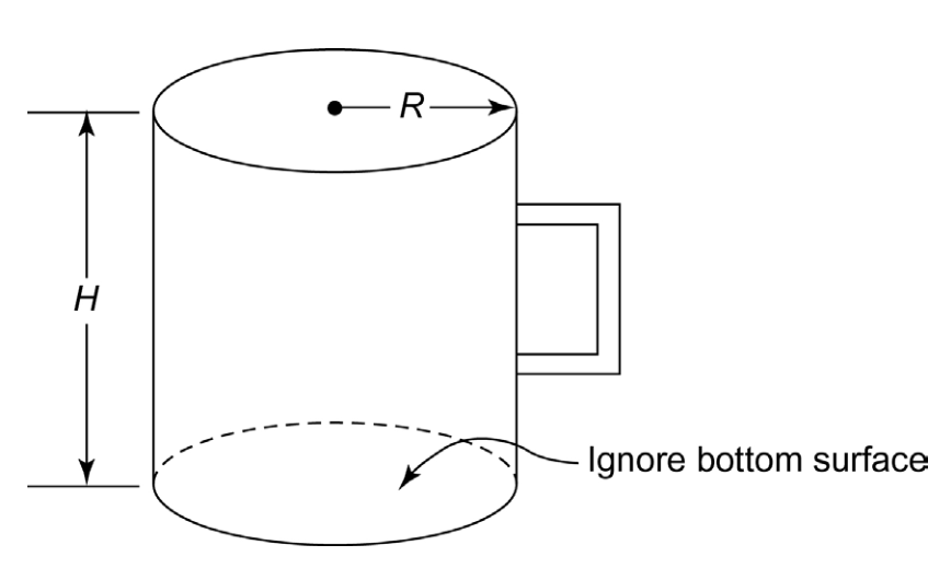
Step 2: Data and Information Collection * The mug has a height \(H\) and a radius \(R\). * There are limitations on the mug’s dimensions and surface area. * Formulas: * Volume of a cylinder: \(V = \pi R^2 H\) * Surface area of the sides: \(A_{sides} = 2\pi R H\) (ignoring the bottom and handle area, as specified in a typical problem statement).

Step 3: Definition of Design Variables * \(x_1 = R\) (radius of the mug, in cm) * \(x_2 = H\) (height of the mug, in cm)

Step 4: Optimization Criterion Maximize the volume of the mug: Maximize \(f(x_1, x_2) = \pi x_1^2 x_2\)

Step 5: Formulation of Constraints 1. Maximum Height Constraint: The height of the mug should be no more than 20 cm. \(x_2 \le 20 \quad \Rightarrow \quad g_1(x_1, x_2) = x_2 - 20 \le 0\) 2. Maximum Radius Constraint: The radius of the mug should be no more than 20 cm. \(x_1 \le 20 \quad \Rightarrow \quad g_2(x_1, x_2) = x_1 - 20 \le 0\) 3. Minimum Radius Constraint: The mug must be at least 5 cm in radius. \(x_1 \ge 5 \quad \Rightarrow \quad g_3(x_1, x_2) = 5 - x_1 \le 0\) 4. Surface Area Constraint: The surface area of the sides must be no greater than 900 cm\(^2\). \(2\pi R H \le 900 \quad \Rightarrow \quad 2\pi x_1 x_2 \le 900\) Rewriting as \(g_j(\mathbf{x}) \le 0\): \(g_4(x_1, x_2) = 2\pi x_1 x_2 - 900 \le 0\) 5. Non-negativity Constraints (Implicit in bounds, but explicitly stated for completeness): \(x_1 \ge 0\) \(x_2 \ge 0\)

Summary of Formulation: Maximize \(f(x_1, x_2) = \pi x_1^2 x_2\) Subject to: \(g_1(x_1, x_2) = x_2 - 20 \le 0\) \(g_2(x_1, x_2) = x_1 - 20 \le 0\) \(g_3(x_1, x_2) = 5 - x_1 \le 0\) \(g_4(x_1, x_2) = 2\pi x_1 x_2 - 900 \le 0\) \(x_1 \ge 0\) \(x_2 \ge 0\)

This concludes our discussion on optimum design problem formulation. Mastering this skill is fundamental, as it dictates the success of all subsequent optimization efforts. In the next lecture, we will explore the Graphical Solution Method and use it to visualize basic optimization concepts, especially for problems with two design variables.