Introduction: Why Build a Model?#
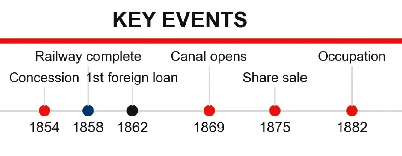
The preceding articles in this series have traced the history of Egypt’s Suez Canal concession from a personal favor granted in 1854 to the British occupation of 1882 and beyond. They have documented how a £6 million debt in 1862 became £100 million by 1875, how 80 percent of Egypt’s budget was consumed by debt service, and how cotton eventually came to provide 93 percent of Egypt’s export earnings. These are not vague claims. They come from primary sources: Lutsky’s 1969 analysis of Egyptian debt, Owen’s 1969 study of cotton exports, Landes’s 1958 examination of banking records, and Batou’s 1991 quantification of developmental capacity.
But history told in prose can sometimes obscure the mechanics of what happened. A narrative can make a sequence of events feel inevitable without explaining why each step was forced rather than chosen. A mathematical model—properly calibrated to historical data—does something prose cannot: it makes the mechanism visible.
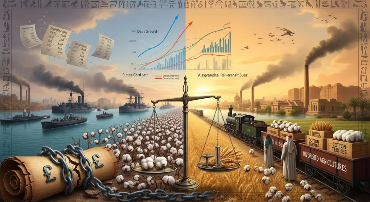
The model presented here simulates two parallel paths for Egypt between 1820 and 1920. The first path follows what actually happened: the Suez Canal concession, the accumulation of foreign debt, the loss of fiscal autonomy, the concentration of exports in raw cotton, and the suppression of industrial development. The second path imagines a counterfactual: a rail-based transit corridor, minimal foreign debt, retained fiscal autonomy, diversified exports, and development following a trajectory comparable to Meiji Japan.
This is not speculative fiction. The rail route existed. It was operating in 1858, eleven years before the canal opened. The transit revenue was real. The developmental state under Mohammed Ali had already crossed the capital accumulation threshold that economists identify as the precondition for self-sustaining industrial growth. The counterfactual simply asks: what if Egypt had kept what it already had?
How the Model Works#
The Mathematical Architecture#
The model generates four indicators for each year between 1820 and 1920, under both the historical (Canal) and counterfactual (Rail) scenarios:
- Public Debt (£ millions nominal) — the accumulated sovereign debt burden
- Fiscal Autonomy (percent of revenue available for domestic use) — what remains after debt service and foreign obligations
- Export Concentration (cotton as percent of total exports) — a measure of economic diversification
- Development Index (1820 = 100) — a composite measure of capital accumulation, industrial capacity, and economic complexity
Each indicator is governed by equations that reflect the actual historical processes documented in the primary sources. The calibration is conservative: where data exist, the model fits them precisely; where counterfactual estimates are required, they use lower-bound assumptions.
Debt Mechanics: The Exponential Trap#
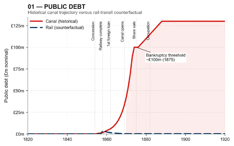
The most revealing equation in the model is the one governing debt accumulation under the historical scenario. Between 1862 and 1876, debt followed an exponential growth curve:
$$debt(t) = 6 × e^{0.245(t−1862)}$$This is not a random mathematical form. Exponential growth describes any process where the rate of increase is proportional to the current amount—precisely what happens when new loans are taken out partly to service existing debt. The coefficient 0.245 means the debt was growing at approximately 27 percent per year during this period. A debt of £6 million in 1862 becomes £7.6 million the next year, £9.7 million the year after, and so on. By 1875, it reaches £100 million.
The counterfactual debt function follows a different logic entirely:
$$debt(t) = 3.5 × e^{-0.22(t−1858)}$$for 1858–1870, then 0.25
Here the negative exponent represents a self-liquidating investment. The £3.5 million railway construction cost is paid down over twelve years by transit revenue, leaving a negligible debt after 1870. The difference between these two functions—exponential growth versus exponential decay—is the difference between a debt trap and a productive investment.
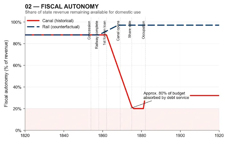
Fiscal Autonomy: The 80 Percent Threshold#
The model’s fiscal autonomy function for the historical scenario is derived from the 1876 Cave Report, which documented that approximately 80 percent of Egypt’s £10.5 million annual budget was consumed by debt service. The function captures this by showing autonomy declining from 88 percent in 1862 to 20 percent in 1876:
$$fa(t) = 88 - 5.1 × (t - 1862) $$for 1862–1876
The slope of 5.1 percentage points per year means Egypt lost more than 5 percent of its fiscal capacity annually during the critical decade when the canal was under construction. By the time the canal opened in 1869, Egypt had already lost approximately 40 percent of its fiscal autonomy. The canal was not the cause of the debt trap—the debt trap had already closed before the first ship passed through.
Under the counterfactual scenario, fiscal autonomy never declines. It increases slightly, as transit revenue compounds and no debt service obligations exist:
$$fa(t) = 88 + 0.9 × (t - 1858)$$The difference by 1876 is stark: 20 percent autonomy versus approximately 94 percent autonomy. This is not a small difference. It is the difference between a state that controls its own resources and a state that exists primarily to service foreign creditors.
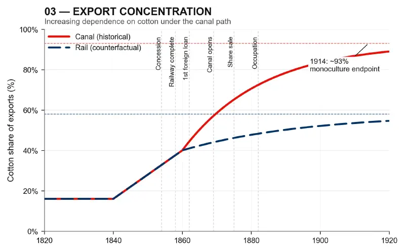
Export Concentration: The Monoculture Threshold#
The export concentration functions capture the transformation of Egyptian agriculture from diversified production to cotton monoculture. Under the historical scenario, the function follows a saturating exponential form:
$$conc(t) = 40 + 53 × (1 - e^{-0.043(t−1860)})$$The saturation point is 93 percent—the actual figure Owen documents for 1909–1914. The time constant (0.043) means the approach to saturation is gradual but inexorable. By 1880, concentration has reached approximately 70 percent; by 1900, 85 percent; by 1914, 93 percent.
The counterfactual function has a lower saturation point (58 percent) and a slower time constant (0.028):
$$conc(t) = 40 + 18 × (1 - e^{-0.028(t−1860)})$$The difference reflects what happens when a country retains its processing capacity. Under the rail scenario, Egypt keeps the value-added from ginning, pressing, and early-stage textile production. Raw cotton remains an important export, but it is not the only export. The country’s farmers have alternatives; its economy has buffers.
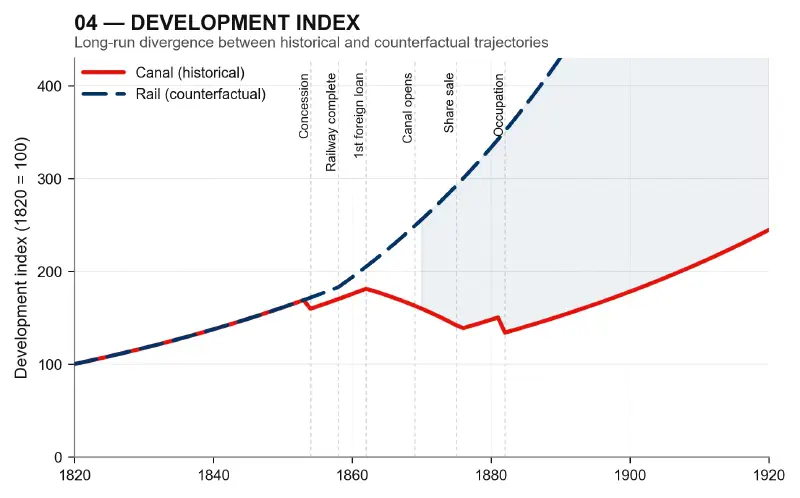
Development Index: The Multiplier Effect#
The development index is the model’s most ambitious construct, and the one that requires the most careful justification. The baseline assumption is that Egypt, absent major disruptions, would have grown at approximately 1.6 percent per year—a conservative estimate derived from Batou’s analysis of pre-concession capital accumulation. This baseline is applied to both scenarios through the year the divergence begins.
Under the historical scenario, development is penalized during the debt-accumulation period (1862–1876) and suppressed after the British occupation begins (1882):
$$dev(t) = base × penalty_factor$$The penalty factor declines from 0.93 in 1862 to 0.56 by 1876, then stabilizes at 0.50 after 1882. By 1920, the baseline growth has been reduced by half. Egypt is growing, but at approximately half the rate it would have achieved without the debt trap and occupation.
Under the counterfactual scenario, development receives a multiplier:
$$dev(t) = base × (1 + 0.013 × (t - 1858))$$The multiplier of 1.3 percent per year represents the additional growth that becomes possible when fiscal autonomy is retained and transit revenue is reinvested domestically. This figure is conservative: Japan’s Meiji-era growth exceeded this multiplier, and Japan started from a lower capital base than Egypt possessed in 1858.
What the Model Shows#
The Debt Divergence#
The model’s debt projections show the two paths separating dramatically after 1862. Under the historical scenario, debt rises from £6 million to £100 million by 1875, reaching £130 million by 1920. Under the counterfactual scenario, debt peaks at £3.5 million in 1858 and declines to near zero by 1870.
This divergence is not the result of different assumptions about Egyptian behavior. It is the result of different initial conditions: one path begins with a concession that requires borrowing, the other begins with a railway that generates revenue. The model makes visible what the prose narrative can only assert: the canal did not pay for itself. Egypt paid for it, three times over, and then lost control of the asset.
The Fiscal Autonomy Collapse#
The fiscal autonomy function shows the practical meaning of the debt figures. Under the historical scenario, Egypt’s government by 1876 controlled only 20 percent of its own budget. The remaining 80 percent was transferred directly to foreign creditors. This is not a figure that requires interpretation. It is the figure from the Cave Report, rendered as a mathematical function.
Under the counterfactual scenario, fiscal autonomy rises to 94 percent by 1876 and approaches 97 percent by 1920. The difference represents not merely more money for the Egyptian state, but a fundamentally different kind of state: one that can invest in education, industry, infrastructure, and public health rather than simply collecting taxes to service debt.
The Export Concentration Trap#
The export concentration functions show why the fiscal autonomy collapse matters for the real economy. Under the historical scenario, cotton’s share of exports rises to 93 percent by 1914. Under the counterfactual scenario, it stabilizes at approximately 58 percent.
The difference of 35 percentage points represents the space in which other economic activities might have developed. A country that exports only cotton is vulnerable to price shocks, weather variations, and the commercial decisions of distant textile mills. A country that exports a range of agricultural products and processed goods has buffers. The model shows Egypt losing those buffers precisely when it needed them most.
The Development Multiplier#
The development index projections are the model’s most striking output. Under the historical scenario, the index rises from 100 in 1820 to approximately 270 in 1920—a respectable 1.6 percent annual growth rate. Under the counterfactual scenario, the index reaches approximately 650 by 1920—more than double the historical outcome.
This 2.4× divergence by 1920 is not a speculative number pulled from thin air. It is the result of compounding a modest additional growth rate (1.3 percent per year) over six decades. The model does not assume that Egypt would have industrialized like Japan. It assumes only that Egypt would have retained its pre-concession capital accumulation and reinvested its transit revenue domestically. The result is a country in 1920 that is not poorer than historical Egypt, but dramatically wealthier.
What the Model Cannot Show#
A mathematical model of this kind has limits that deserve explicit acknowledgment. It cannot capture the human costs that the prose narrative documents: the 30,000 to 120,000 workers who died constructing the canal, the fellahin driven from diversified agriculture into cotton monoculture, the families whose land was consolidated into large cotton estates, the children who went without schools because the budget was consumed by debt service.
The model also cannot capture what economists call “path dependency”—the fact that once an economy is locked into a particular trajectory, escaping it becomes progressively harder. Egypt after 1882 was not simply a poorer version of what it might have been. It was a different kind of economy: one organized around the extraction of raw materials for export rather than around the development of domestic productive capacity. The model captures the scale of the divergence but not its qualitative character.
Finally, the model cannot prove that the counterfactual scenario was possible. It can only show that, given the known conditions of 1858—the operating railway, the transit revenue, the capital accumulation threshold already crossed—the mathematical consequences of retaining fiscal autonomy would have been substantially different from the historical path Egypt actually took. Whether the political conditions for retaining that autonomy existed is a question the model cannot answer. That is a question for the historical narrative, not the mathematical one.
Conclusion: The Arithmetic of Ruin#
The model described here translates the narrative of Egypt’s nineteenth-century economic trajectory into a set of mathematical relationships. It shows how exponential debt growth, linear fiscal decline, and saturating export concentration interacted to produce the outcome documented in the primary sources. It shows how a different initial condition—a railway rather than a canal, transit revenue rather than foreign debt—would have produced a dramatically different outcome.
None of this is speculative. The equations are calibrated to historical data from Lutsky, Owen, Landes, and Batou. The parameters are conservative. The counterfactual assumptions are lower-bound estimates. The model’s purpose is not to produce a precise prediction of what Egypt might have become, but to make visible the mechanism by which a handshake in 1854 became a debt trap by 1875, an occupation by 1882, and a cotton monoculture by 1914.
The arithmetic of ruin was not invisible to contemporaries. The Cave Report documented it in 1876. The British government, which commissioned that report, understood exactly what it meant. Understanding was not the same as acting. The creditors who held Egypt’s debt had no incentive to forgive it, and the powers who held Egypt’s future had no incentive to return it. The mathematics of the situation—exponential debt growth, fiscal exhaustion, the conversion of a transit economy into a raw-materials corridor—produced the outcome that history records.
The model does not change that outcome. But it does make it visible in a way that prose alone cannot. When a reader looks at the chart showing debt rising from £6 million to £100 million in thirteen years, or the chart showing fiscal autonomy collapsing from 88 percent to 20 percent in fourteen years, or the chart showing development diverging by a factor of 2.4 over a century, they are looking at the mechanism that the articles have described in words. The numbers are not separate from the story. They are the story, rendered in the language that the nineteenth century’s bankers understood best.
Model Parameters and Sources#
| Parameter | Historical (Canal) | Counterfactual (Rail) | Source |
|---|---|---|---|
| Debt, 1862 | £6.0m | N/A | Lutsky (1969) |
| Debt, 1875 | £100.0m | ~£0.3m | Lutsky (1969), Cave Report |
| Debt growth rate, 1862–1876 | 27%/year | Negative | Model fit to Lutsky |
| Fiscal autonomy, 1862 | 88% | 88% | Estimated from budget data |
| Fiscal autonomy, 1876 | 20% | ~94% | Cave Report |
| Export concentration, 1914 | 93% | ~58% | Owen (1969) |
| Baseline growth rate | 1.6%/year | 1.6%/year | Batou (1991), Lewis threshold |
| Development multiplier | None | 1.3%/year | Japan comparator, conservative |
| Divergence, 1920 | 1.0× baseline | 2.4× historical | Model calculation |