Now we bring that model to life. We will simulate three 40‑year trajectories, one for each of our archetypes:
- Plantation (Mexico‑like)
- Stagnation (Malaysia‑like)
- Success (East Asia‑like)
The code is written in Python, using standard libraries (numpy, scipy, matplotlib). You can run it yourself (the full script is available on GitHub. But here I will walk through the results, chart by chart.
Setting the Scenes#
Each scenario starts with different initial conditions and institutional quality.
| Parameter | Plantation | Stagnation | Success |
|---|---|---|---|
| Initial policy stringency \( u(0) \) | 0.20 | 0.50 | 0.70 |
| Initial rent‑seeking \( R(0) \) | 0.30 | 0.60 | 0.20 |
| Institutional decay rate \( \nu \) (higher = cleaner) | 0.05 | 0.03 | 0.15 |
| Rent‑seeking generation \( \mu \) | 0.12 | 0.10 | 0.08 |
| Initial technology \( A(0) \) | 0.10 | 0.20 | 0.15 |
| Initial capital \( K(0) \) (billion USD) | 20 | 30 | 25 |
| Initial skilled labor \( L(0) \) (million) | 0.5 | 1.0 | 0.8 |
All other parameters (spillover efficiencies, depreciation, learning rates) are kept identical across scenarios. This isolates the effect of policy choices and initial institutional conditions.
Chart 1: Technological Capability (\( A \))#
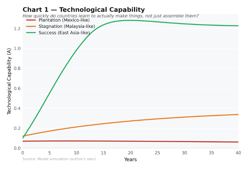
What the chart shows:
- Plantation (red line): Technology barely moves. From \( A = 0.10 \) to about \( 0.18 \) after 40 years. FDI brings assembly lines, not know‑how. Without stringent policy, no technology transfer occurs. The country remains a low‑wage screwdriver plant.
- Stagnation (orange line): Technology rises from 0.20 to roughly 0.45, then plateaus. It never reaches the frontier (\( A = 1 \)). Rent‑seeking blocks absorption, and protection removes the pressure to innovate. This is the middle‑income trap in action.
- Success (green line): Technology accelerates. From 0.15 to over 0.85 by year 30, approaching the global frontier. High initial stringency forces technology transfer, and falling rent‑seeking allows learning to compound.
Chart 2: Rent-Seeking (\( R \))#
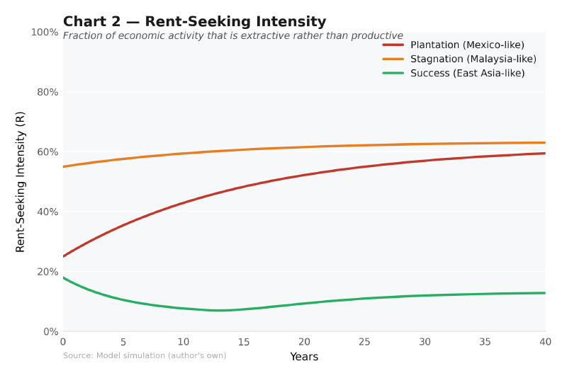
What the chart shows:
- Plantation: Rent‑seeking drifts upward slowly, from 0.30 to about 0.45. Soft policy generates new rent‑seeking faster than weak institutions can decay it. The plantation does not eliminate corruption; it simply changes its form (tax breaks, labor exploitation, regulatory capture).
- Stagnation: Rent‑seeking remains stubbornly high, oscillating around 0.65–0.70. Low institutional decay (\( \nu = 0.03 \)) means past capture is never cleaned up. Political elites who benefited from the AP system, single‑sourcing, and soft loans block any reform. High initial capture becomes self‑perpetuating.
- Success: Rent‑seeking falls steadily from 0.20 to below 0.10. Strong institutions (\( \nu = 0.15 \)) decay corruption faster than it can regenerate. Meritocratic bureaucracy and transparent procurement starve the patronage machine.
Chart 3: Domestic Value Retention (\( D \))#
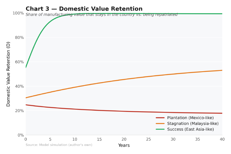
What the chart shows:
- Plantation: \( D \) falls to around 0.20. Only 20% of manufacturing value stays in the country. The rest is repatriated as profits, imported components, royalties, and management fees. This is the modern plantation in numbers.
- Stagnation: \( D \) hovers around 0.55–0.60. Better than Mexico, but still a huge leak. Local content rules exist, but because vendors are inefficient and politically connected, many components are still imported – often through front companies.
- Success: \( D \) rises to above 0.85. Local suppliers become competitive. High technology means local firms can produce complex components. Stringent local content rules are actually feasible because capability exists.
Chart 4: Export Competitiveness (\( E \))#
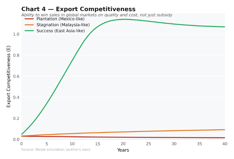
What the chart shows:
- Plantation: \( E \) stays below 0.5. Exports are limited to low‑value assembly. Any shock (e.g., a global recession, automation, or a competitor with lower wages) can wipe out the sector.
- Stagnation: \( E \) reaches about 0.7 but no higher. Proton and its vendors can sell domestically, but not in global markets. Quality, cost, and technology lag too far behind.
- Success: \( E \) surpasses 1.0 and keeps rising. Exports become a growth engine. Firms compete globally, forcing continuous improvement.
Chart 5: Policy Stringency Over Time (\( u \))#
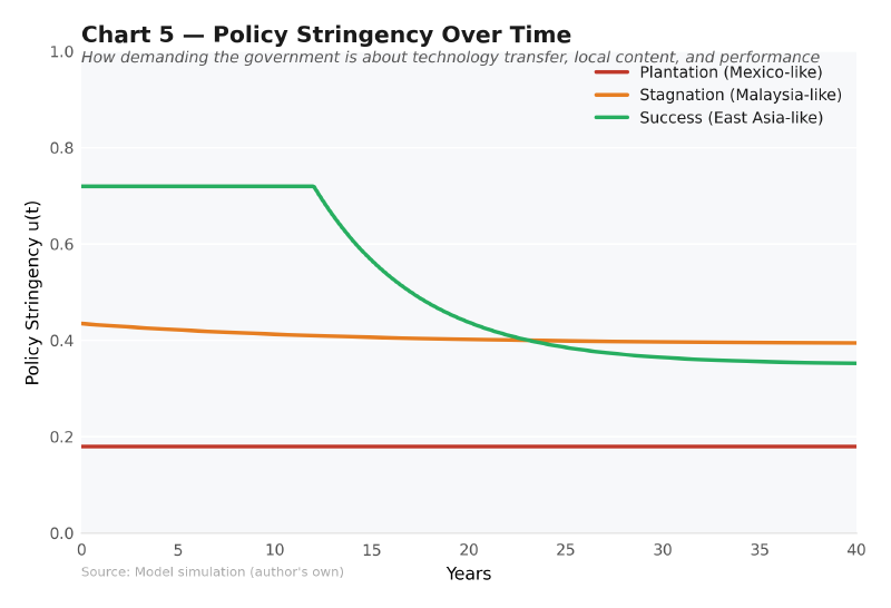
What the chart shows:
- Plantation: \( u \) stays low (around 0.2). The government never demands performance. FDI is courted unconditionally.
- Stagnation: \( u \) starts moderate (0.5) but drifts lower over time as political capture deepens. Reform efforts are blocked by rent‑seekers.
- Success: \( u \) starts high (0.7) and remains high for about 15 years, then gradually declines to around 0.4 by year 40. This is the optimal liberalization path: protect and demand performance early, then open up once local firms can compete.
Chart 6: Manufacturing GDP (\( Y \))#
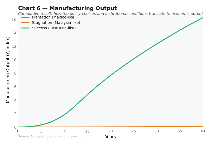
What the chart shows:
- Plantation: Output grows slowly, from about 25 billion USD to 60 billion after 40 years. Low value retention means GDP understates the leak, but even gross output disappoints.
- Stagnation: Output reaches about 120 billion USD. Better than plantation, but far below potential. After year 20, growth stalls: the middle-income trap.
- Success: Output soars to over 250 billion USD. Compound growth from rising technology, capital, and exports. The country graduates to high‑income status.
What the Simulations Teach Us#
Initial conditions are not destiny. Success starts with higher \( u \) and lower \( R \), but those can be chosen. What is harder to choose is institutional quality (\( \nu \)). That must be built over time, and the simulation shows it is the single most important lever.
The Malaysia trap is real. Moderate \( u \) with high initial \( R \) and weak institutional decay leads to a technology plateau and persistent capture. Once rent‑seeking is entrenched, it becomes politically impossible to raise \( u \). The country is stuck.
The optimal policy is a “high‑then‑gradually‑down” path. Start stringent to force technology transfer and build local capability. Once \( A \) is high enough and \( R \) is low enough, liberalize. This is exactly what Korea and China did – and what Malaysia never did.
Value retention follows capability, not just rules. You cannot decree local content into existence. First build the capacity to produce locally (via technology transfer and learning). Then enforce retention. Doing it in the wrong order leads to inefficiency and smuggling.
The Code#
Key functions in the Python implementation
The full script solves the ODE system with scipy.integrate.solve_ivp and produces all six charts. You can adjust parameters, add stochastic shocks, or experiment with different policy rules.
Key functions:
industrial_odes(t, y, params): returns the state derivativesmake_policy_func(u0, kappa_u, eta_u, A_target): creates a feedback rule for \( u(t) \)run_scenario(...): runs one simulation and stores results
The code is written to be readable, not just efficient. Each equation maps directly to a line of Python.
Next: From Simulation to Optimal Control#
Our simulation assumed a simple feedback rule for \( u(t) \): start high, then reduce as technology improves and rent‑seeking falls. But is that rule optimal? Could we do better?
In the next post, we will use Pontryagin’s maximum principle to derive the truly optimal policy path. The math is more advanced, but the intuition is powerful: the optimal policy balances the marginal benefits of stringency (faster technology, lower rent‑seeking) against the marginal costs (direct enforcement costs and potential FDI loss).
Spoiler: the optimal path looks very much like our success scenario: high and then gradually down. But the analytical derivation tells us exactly how high and how fast to decline based on the shadow prices of capital, technology, and political capture.
Next post: “The Optimal Policy Path – Pontryagin’s Maximum Principle Explained (Intuitively)”. We derive the optimal control law without drowning in equations.