But stories alone cannot guide policy. They cannot tell us how much protection is too much, how long it should last, or when to liberalize. For that, we need a model: a simplified mathematical representation of the key forces at work.
This post introduces such a model. Do not fear the equations. They are not here to intimidate. They are here to clarify. And by the end, you will see how the three paths (plantation, stagnation, success) emerge naturally from different policy choices and institutional conditions.
The Core Variables#
We focus on five quantities that evolve over time:
| Symbol | Meaning |
|---|---|
| \( K(t) \) | Capital stock in manufacturing (factories, machinery, infrastructure) |
| \( A(t) \) | Technological capability (how advanced your production methods are) |
| \( R(t) \) | Rent-seeking / political capture (0 = clean, 1 = fully captured) |
| \( D(t) \) | Domestic value retention (share of value that stays in the country) |
| \( E(t) \) | Export competitiveness (ability to sell abroad) |
The government controls one key lever: policy stringency \( u(t) \), which ranges from 0 to 1.
- \( u = 0 \): complete laissez-faire, no demands on FDI, no protection for local firms (Mexico)
- \( u = 1 \): maximum stringency, demanding technology transfer, local content, and export performance, with strong protection (early Korea)
- Moderate \( u \): somewhere in between, but if institutions are weak, capture can still occur (Malaysia)
The Dynamics in Plain English#
Before we write equations, let me describe what happens in words.
Capital grows from domestic savings, foreign investment, and the spillover benefits of FDI. But rent-seeking blocks those spillovers: when politically connected elites capture the benefits, new investment does not translate into productive capital.
Technology improves through two channels: learning-by-doing (the more you produce, the better you get) and technology transfer from FDI. But rent-seeking also blocks technology absorption: if engineers are hired based on connections rather than skill, learning suffers.
Rent-seeking itself is not fixed. It grows when policy is soft (because elites can extract without consequence) and decays when institutions are strong (anti-corruption, meritocracy). But once the economy grows large, powerful groups may demand even more rents, a feedback loop that can trap a country.
Domestic value retention is the fraction of output that stays home. It is high when policy is stringent (forcing local sourcing) and when technology is advanced (so locals can actually produce high-value components). It is low under laissez-faire, where MNCs simply import everything and repatriate profits.
Export competitiveness rises with technology and falls with rent-seeking. A corrupt, technologically backward country cannot sell abroad except as a low-wage assembly platform.
The Equations (Simplified)#
Now let me write the core relationships. Do not try to memorize them. Just see the structure.
Capital accumulation:
\[ \frac{dK}{dt} = sY - \delta K + \sigma u (1 - \phi R) F \]- \( sY \): savings from manufacturing output
- \( \delta K \): depreciation
- Last term: FDI contributes to capital, but only if policy stringency \( u \) is high, and rent-seeking \( R \) blocks it (via \( \phi \)).
Technology growth:
\[ \frac{dA}{dt} = \beta u (1 - \theta R) + \text{(learning-by-doing)} - \lambda A \]- First term: technology transfer from FDI, boosted by stringent policy and blocked by rent-seeking
- Second term (not fully written): learning from production
- Third term: technology obsolescence
Rent-seeking dynamics:
\[ \frac{dR}{dt} = \mu (1 - u) - \nu R + \xi R (1 - e^{-\eta Y}) \]- Soft policy (\( u \) low) generates rent-seeking (\( \mu \))
- Strong institutions (\( \nu \) high) decay rent-seeking
- Growing output \( Y \) can also feed rent-seeking (success attracts parasites)
Domestic value retention (algebraic):
\[ D = \frac{1}{1 + \psi (1-u) e^{-\xi A}} \]- When \( u \) is high or \( A \) is high, \( D \) approaches 1 (all value stays)
- When \( u \) is low and \( A \) is low, \( D \) falls toward \( 1/(1+\psi) \), the plantation floor
Export competitiveness (algebraic):
\[ E = \frac{A (1-R)}{1 + \omega e^{-\eta K}} \]- Rises with technology and falls with rent-seeking
- Also benefits from capital scale (larger \( K \) lowers the denominator)
Output:
\[ Y = K^{\alpha} (A L)^{1-\alpha} \cdot D \cdot E \]- Cobb-Douglas production, then multiplied by value retention and export competitiveness (which affect realized income)
The Three Scenarios in the Model#
By choosing different initial conditions and institutional parameters, the model reproduces our three paths.
1. Plantation (Mexico-like)#
- Low initial policy stringency \( u(0) = 0.2 \)
- Weak institutions (moderate \( \nu \), but soft policy keeps \( R \) moderate)
- FDI flows in, but technology transfer is minimal (\( A \) stays low)
- Value retention \( D \) falls to ~0.2, the plantation trap
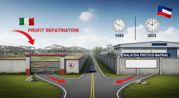
2. Stagnation (Malaysia-like)#
- Moderate initial stringency \( u(0) = 0.5 \)
- But high initial rent-seeking \( R(0) = 0.6 \) and weak institutional decay (\( \nu \) low)
- Protection exists, but capture blocks technology absorption
- Technology plateaus around \( A = 0.4 \), exports never take off, and \( R \) stays high
3. Success (East Asia-like)#
- High initial stringency \( u(0) = 0.7 \)
- Low initial rent-seeking \( R(0) = 0.2 \) and strong institutions (\( \nu \) high)
- Technology accelerates, rent-seeking declines, value retention stays high
- As \( A \) approaches the frontier, policy can gradually liberalize (reduce \( u \))
What the Model Teaches Us#
Even before we run simulations (next post), the model yields three profound insights:
1. There is a narrow corridor for success.
Too low \( u \) → plantation. Moderate \( u \) but high initial \( R \) → capture. High \( u \) with strong institutions → success. The corridor is narrow because both the plantation and capture traps are self-reinforcing.
2. Initial conditions matter enormously.
If a country starts with high rent-seeking (say, \( R(0) > 0.5 \)), it may be impossible to escape the capture trap, because the elites who benefit from soft policy will block any move to high stringency. This is the Malaysia problem: past decisions create path dependence.
3. Institutions are the ultimate lever.
The parameter \( \nu \) (rate at which rent-seeking decays) is not given by nature. It is built through anti-corruption agencies, meritocratic civil service, transparent procurement, and independent courts. Without institutional quality, even a well-designed policy will be captured.
From Model to Simulation#
In the next post, we will translate these equations into Python code and simulate the three scenarios over 40 years. You will see the technology gap close, or fail to close, in vivid charts. You will watch rent-seeking rise or fall. And you will understand, quantitatively, why Malaysia and Mexico got stuck while Korea and China broke through.
But before we run the code, remember: the model is a simplification. Real countries are messier. But a good model, like a good map, helps you navigate even if it leaves out some trees.
The key takeaway from this post is simple:
In the next post, we will see the numbers.
Next post: “Simulating the Future – Python Code and Scenario Analysis”. We will run the model, generate charts, and compare the three trajectories year by year.